Theory of Operation

Density measurements for photography and graphic technology is officially based upon the following standards documents [1]:

• ISO 5-1:2009 - Geometry and functional notation

• ISO 5-2:2009 - Geometric conditions for transmittance density

• ISO 5-3:2009 - Spectral conditions

• ISO 5-4:2009 - Geometric conditions for reflection density

Warning

The text in this section is currently based on the Printalyzer Densitometer (DPD-100) and/or is a work in progress. While the theory of operation for basic density calculations is unchanged for the Printalyzer UV/VIS Densitometer (DPD-105), there have been significant changes to the calibration process and the sensor head design.

Basic Calculations

Reflection Density

Reflection density is typically defined by the following formula:

\(D_R = -log_{10} R\)

In this formula, “R” is defined as the reflectance factor. That means it is the ratio of light detected by the sensor as reflecting off of the target material, to light that would be detected if the target was a perfectly reflecting and perfectly diffusing material.

In practice, the reflection calculations are based on using two reference measurements to draw a line in logarithmic space. The location of the target measurement along this line then determines its density.

The inputs to this calculation are:

• \(V_{target}\): Sensor measurement of the target material

• \(V_{hi}\): Sensor measurement of the CAL-HI reference

• \(D_{hi}\): Known density of the CAL-HI reference

• \(V_{lo}\): Sensor measurement of the CAL-LO reference

• \(D_{lo}\): Known density of the CAL-LO reference

First, all the input measurements are converted into logarithmic space:

\begin{align*} L_{target} &= log_{10} V_{target} \\ L_{hi} &= log_{10} V_{hi} \\ L_{lo} &= log_{10} V_{lo} \end{align*}

Then the slope of the line connecting CAL-HI and CAL-LO is determined:

\[m = \frac{D_{hi} - D_{lo}}{L_{hi} - L_{lo}}\]

Finally, the measured density is calculated:

\[D_{target} = (m * (L_{target} - L_{lo})) + D_{lo}\]

Note: An alternative approach would be to use just the CAL-LO properties to determine what a perfect reflection reading would be, then use that value in the original density formula. In theory, this would yield the same answer. In practice however, due to limited density precision of the reference strips, the results would be slightly different. For this reason, the single reference point approach is only viable when using laboratory grade reflectance standards.

Transmission Density

Transmission density is typically defined by the following formula:

\(D_T = -log_{10} T\)

In this formula, “T” is defined as the transmittance factor. That means it is the ratio of light detected by the sensor as passing through the target material, to light that would be detected if the path from the light source to the sensor was unobstructed.

In practice, the transmission calculations are based on using two reference measurements to compensate for any sensor error. One is the measurement of an unobstructed light path, while the other is the measurement of a high density reference material.

The inputs to this calculation are:

• \(V_{target}\): Sensor measurement of the target material

• \(V_{hi}\): Sensor measurement of the CAL-HI reference

• \(D_{hi}\): Known density of the CAL-HI reference

• \(V_{zero}\): Sensor measurement of an unobstructed light path

First, calculate the measured target and CAL-HI densities relative to the unobstructed light reading:

\begin{align*} M_{hi} &= -log_{10}\left(\frac{V_{hi}}{V_{zero}}\right) \\ M_{d} &= -log_{10}\left(\frac{V_{target}}{V_{zero}}\right) \end{align*}

Then calculate the adjustment factor based on the known density of our CAL-HI reference:

\[F_{adj} = \frac{D_{hi}}{M_{hi}}\]

Finally, put these together to calculate the transmission density:

\[D_{target} = M_{d} * F_{adj}\]

Preparing Readings

Before any of the above calculations can be performed, the raw sensor readings must first be converted into a normalized and corrected form. This conversion takes into account a number of sensor properties to arrive at a floating point value that is independent of the sensor’s measurement settings and is corrected for any deviations in the sensor’s response curve.

This process consists of the following steps:

• Start with the raw sensor reading and parameters

• Convert to basic counts, which factor in gain and integration time

• Apply temperature correction, which is based on the ambient temperature inside the sensor head

As the input to each of these steps depends on the output of the previous steps, calibration is performed in the same order that the corrections are applied. All the calibration measurements required for this process are performed as part of device manufacturing, as they typically require conditions, instruments, or materials not provided with the device itself.

Gain Calibration

Because of the wide range of light values that need to be measured, the gain setting of the sensor cannot be kept constant across all measurements. Therefore, the current gain setting needs to be factored into any calculations that compare sensor readings.

The datasheet for the sensor does not provide exact values for these gain settings, but rather a range that can be expected.

Table 1 Sensor Datasheet Gain Values

Setting	Min	Typical	Max
0.5x	0.47	0.51	0.55
1x	0.96	1.03	1.11
2x	1.91	2.03	2.15
4x	3.83	4.04	4.24
8x	7.92	8.24	8.57
16x	15.42	16.06	16.71
32x	30.84	32.08	33.42
64x	61.24	63.68	66.32
128x	-	128	-
256x	227.84	247.04	264.96

To determine the actual values for these gain settings, or as close to them as we can get, a calibration process is required. This process is mostly automated, triggered by the desktop application. It works by leaving the device unattended with the sensor head held closed by a weight or strap, while a series of independent raw measurements are performed. For the sake of consistency, gain calibration is typically performed at an ambient temperature of approximarely 20°C.

For each adjacent pair of gain settings, the following process is performed:

• Determine the appropriate light brightness to get a good reading at the higher gain, without saturation

• Measure the light at the lower gain

• Meadure the light at the higher gain

• Calculate the ratio between these two gains

Between each step there is a cooldown cycle, to ensure consistent readings.

Once these readings are complete, we end up with a table such as this:

Table 2 Example Gain Pair Ratios

Pair	Ratio
\(g_1/g_0\)	2.02896631
\(g_2/g_1\)	1.97246370
\(g_3/g_2\)	1.99469659
\(g_4/g_3\)	1.93522371
\(g_5/g_4\)	1.97304038
\(g_6/g_5\)	1.99064724
\(g_7/g_6\)	1.98492706
\(g_8/g_7\)	2.00797774
\(g_9/g_8\)	1.90163819

We then take the highest gain we can measure at full brightness without sensor saturation, set that as the reference gain, and calculate the actual gain table as follows:

Table 3 Example Measured Gain Table

Gain	Setting	Actual Value
\(g_0\)	0.5x	0.517843
\(g_1\)	1x	1.050686
\(g_2\)	2x	2.072440
\(g_3\)	4x	4.133889
\(g_4\)	8x	8.000000
\(g_5\)	16x	15.784323
\(g_6\)	32x	31.421019
\(g_7\)	64x	62.368431
\(g_8\)	128x	125.234421
\(g_9\)	256x	238.150558

Converting to Basic Counts

Raw sensor readings cannot be compared directly, because there are a number of variables that need to be taken into consideration. The process of incorporating these into the result transforms that result from a raw reading into something referred to as “basic counts.”

The inputs to this conversion are as follows:

• \(V_{raw}\): Raw 32-bit integer representing the output of the sensor’s analog-to-digital converter (ADC)

• \(A_{time}\): Sensor integration time, in milliseconds [2]

• \(A_{gain}\): Sensor gain value, for the active gain setting, as determined above

The conversion itself is then as follows:

\begin{align*} V_{basic} &= \frac{V_{raw} / 16}{A_{time} \cdot A_{gain}} \end{align*}

Temperature Calibration

[TODO]

Temperature Correction

[TODO]

Sensor Head Design

The sensor head is designed to support both reflection and transmission measurements from a single sensor element, using multiple light sources. It is articulated using a hinge mechanism that brings the two halves of the unit to a repeatable alignment and parallel position, when an object no thicker than a normal piece of photographic film or paper is placed in-between.

For reflection measurements, the light source consists of four 3000K white light-emitting diodes (LEDs) arranged and directed so that they shine at a 45° angle to the target. This arrangement was chosen to ensure even illumination regardless of surface or alignment imperfections, and because it provides a converging cross-hair effect when positioning a material to be measured. The LEDs are driven with a constant current that is matched between all four of them to ensure even illumination.

For transmission measurements, the light source consists of four 3000K white LEDs and a single 385nm UV LED positioned below a flashed opal diffuser in the base of the unit. This arrangement provides the same illumination effect as if both a white and a UV LED were occupying the same spot. The white LEDs are driven by a constant current driver that is matched between all for of them to ensure even illumination, while the UV LED has its own separate constant current driver.

The light path towards the sensor itself, within the sensor head, consists of a focusing lens followed by a UVFS diffuser. These help tighten the measurement spot, improve the amount of light that reaches the sensor, and even out the light hitting the surface of the sensor itself.

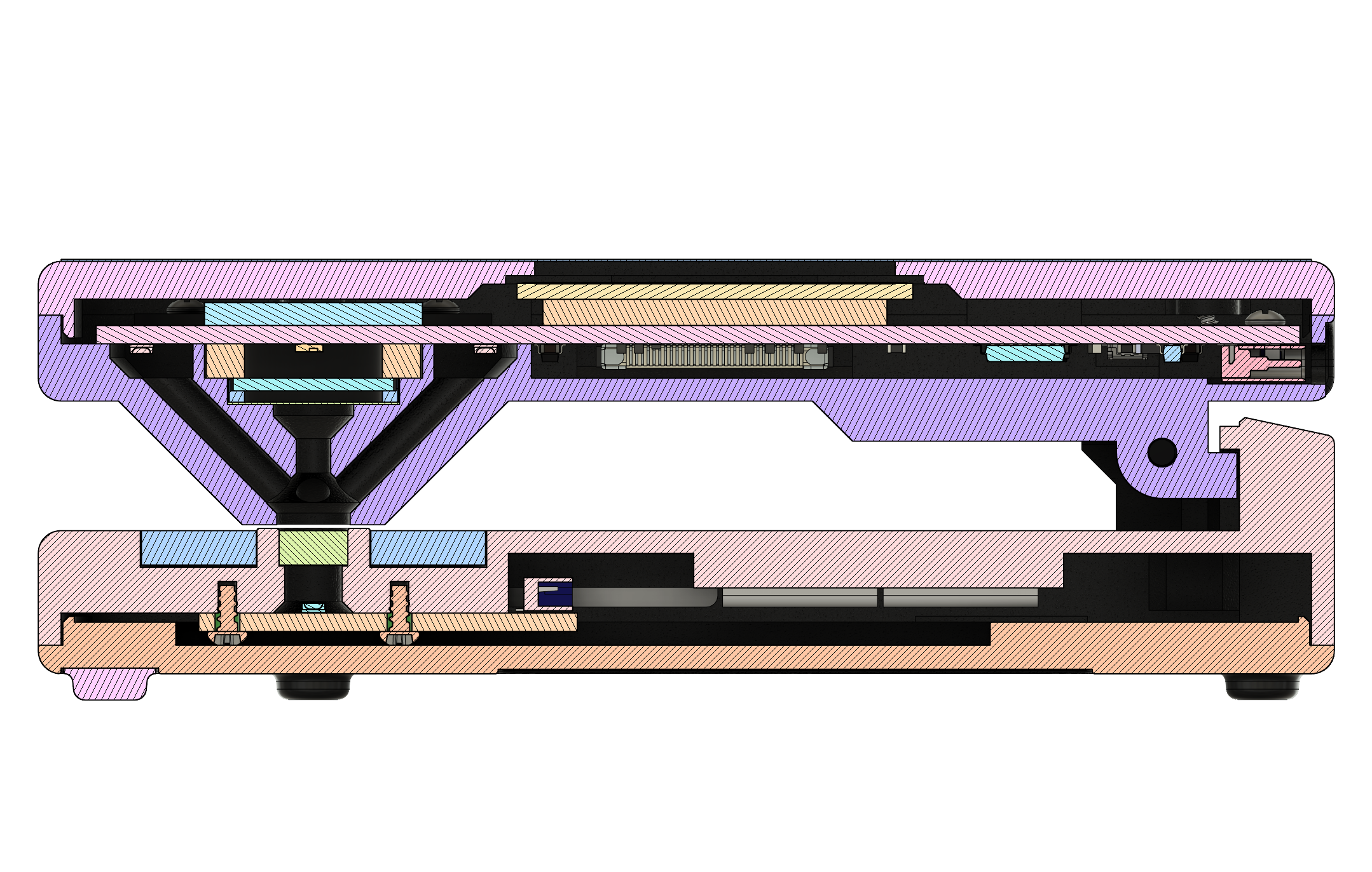
Fig. 9 Cross-section (side view)

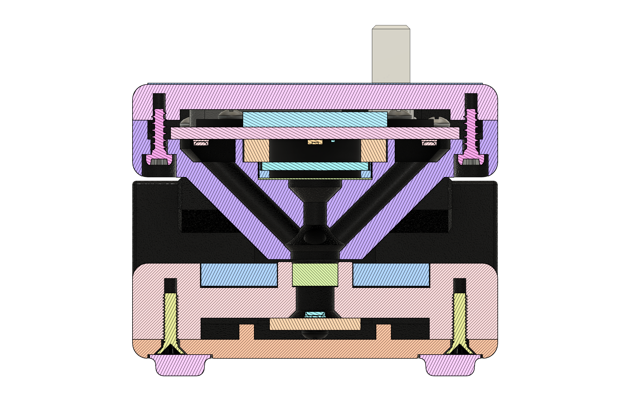
Fig. 10 Cross-section (sensor head)

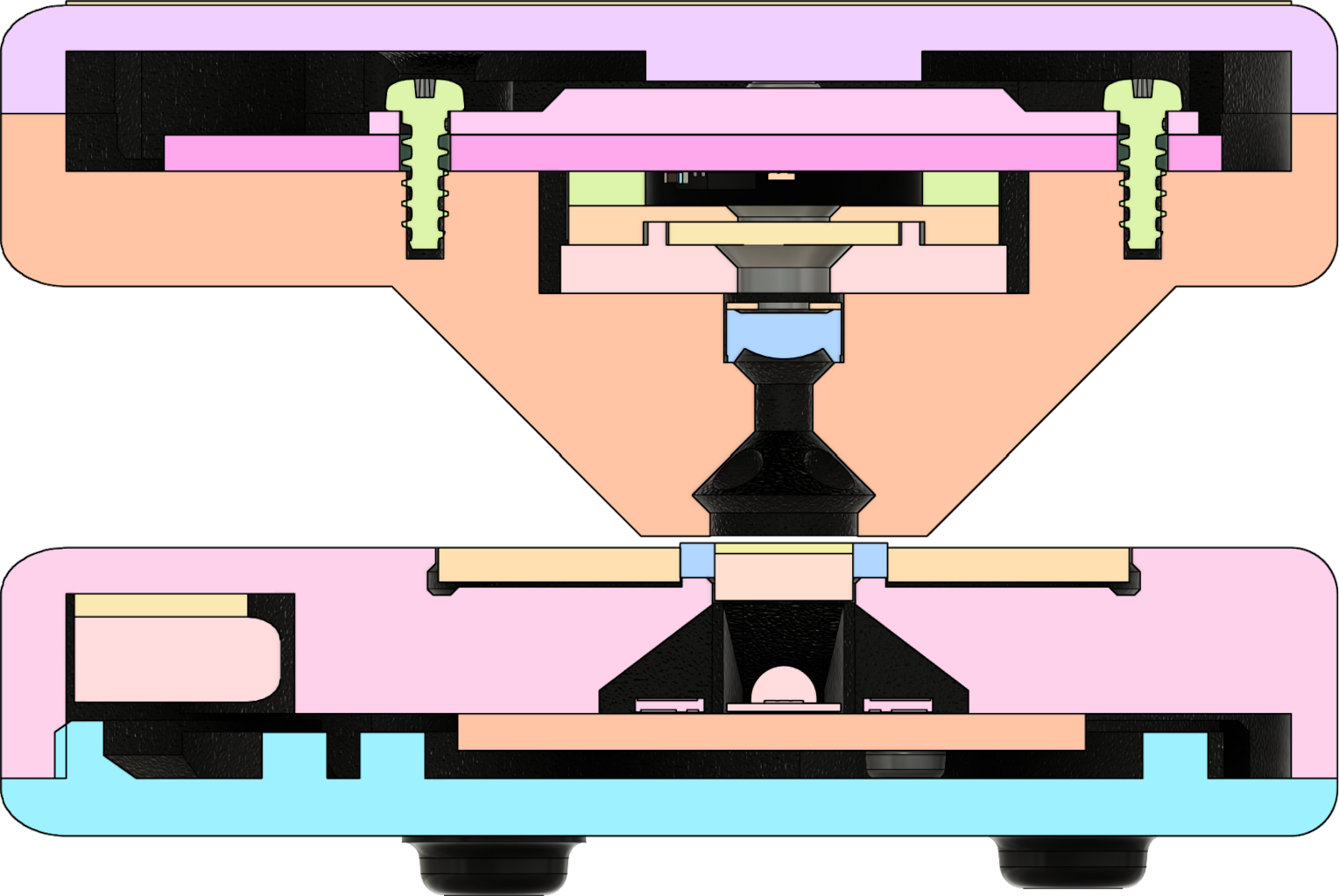
Fig. 11 Cross-section (sensor head, 45° angle)

Response Spectrum

[TODO: Update spectrum description]

The ISO specification for photographic density provides spectral conditions for each kind of density measurement. To reduce cost and increase ease of part sourcing, the sensor used in this device is an off-the-shelf component that was not designed with these conditions in mind. While it is close, it does not exactly match. That being said, when the response curve from the sensor’s datasheet is combined with the transmission curve of the UV-IR cut filter, the combined sensitivity spectrum can be seen in Fig. 12.

Fig. 12 Spectral response of the light sensor

It should be noted that because the sensor head’s spectral response only approximates the ISO 5-3:2009 Visual Spectrum specification, and because modern LED-based light sources do not have the same full spectrum emissions as a tungsten lamp, the most consistent results will be achieved on normal black and white photographic materials. If the measurement target has a strong shift to the blue or red side of the light spectrum, results may no longer match up.

Temperature Performance

[TODO: Remove or rewrite]

As part of pre-production device testing, the densitometer was subjected to a wide range of thermal conditions to determine their effect on density measurements. These tests consisted of a repeatable temperature ramp from 0°C through 45°C, and were conducted with a wide range of high and low density materials secured within the device’s measurement target area. The readings were normalized around 25°C, and the measurement errors from the test can be seen in Fig. 13. The conclusion from these tests was that temperature has a very minimal effect across a reasonably large range.

Fig. 13 Temperature sensitivity of density readings

It should be noted that the lines on this graph with the most jagged or inconsistent results were from high density transmission targets where the measurement resolution is relatively low. Due to the logarithmic nature of the scale, it would not be practical to increase the brightness of the light source by a large enough amount to compensate for this.

Footnotes

[1]

The ISO standards for density were preceded by the following ANSI standards: PH 2.16, PH 2.17, PH 2.18, and PH 2.19. Older product specifications are likely to cite these instead.

[2]

To avoid the need to calibrate the integration time, all readings are taken with the same value for this variable.