Theory of Operation

Density measurements for photography and graphic technology is officially based upon the following standards documents 1:

• ISO 5-1:2009 - Geometry and functional notation

• ISO 5-2:2009 - Geometric conditions for transmittance density

• ISO 5-3:2009 - Spectral conditions

• ISO 5-4:2009 - Geometric conditions for reflection density

This section will eventually contain an in-depth description of the design and functionality of the device, as well as the various formulas used in the density calculations.

Basic Calculations

Reflection Density

Reflection density is typically defined by the following formula:

\(D_R = -log_{10} R\)

In this formula, “R” is defined as the reflectance factor. That means it is the ratio of light detected by the sensor as reflecting off of the target material, to light that would be detected if the target was a perfectly reflecting and perfectly diffusing material.

In practice, the reflection calculations are based on using two reference measurements to draw a line in logarithmic space. The location of the target measurement along this line then determines its density.

The inputs to this calculation are:

• \(V_{target}\): Sensor measurement of the target material

• \(V_{hi}\): Sensor measurement of the CAL-HI reference

• \(D_{hi}\): Known density of the CAL-HI reference

• \(V_{lo}\): Sensor measurement of the CAL-LO reference

• \(D_{lo}\): Known density of the CAL-LO reference

First, all the input measurements are converted into logarithmic space:

\begin{align*} L_{target} &= log_{10} V_{target} \\ L_{hi} &= log_{10} V_{hi} \\ L_{lo} &= log_{10} V_{lo} \end{align*}

Then the slope of the line connecting CAL-HI and CAL-LO is determined:

\[m = \frac{D_{hi} - D_{lo}}{L_{hi} - L_{lo}}\]

Finally, the measured density is calculated:

\[D_{target} = (m * (L_{target} - L_{lo})) + D_{lo}\]

Note: An alternative approach would be to use the CAL-LO properties to determine what a perfect reflection reading would be, then use that value in the original density formula. In theory, this would yield the same answer. In practice however, due to the side effects of floating point calculations, the results would be slightly different.

Transmission Density

Transmission density is typically defined by the following formula:

\(D_T = -log_{10} T\)

In this formula, “T” is defined as the transmittance factor. That means it is the ratio of light detected by the sensor as passing through the target material, to light that would be detected if the path from the light source to the sensor was unobstructed.

In practice, the transmission calculations are based on using two reference measurements to compensate for any sensor error. One is the measurement of an unobstructed light path, while the other is the measurement of a high density reference material.

The inputs to this calculation are:

• \(V_{target}\): Sensor measurement of the target material

• \(V_{hi}\): Sensor measurement of the CAL-HI reference

• \(D_{hi}\): Known density of the CAL-HI reference

• \(V_{zero}\): Sensor measurement of an unobstructed light path

First, calculate the measured target and CAL-HI densities relative to the unobstructed light reading:

\begin{align*} M_{hi} &= -log_{10}\left(\frac{V_{hi}}{V_{zero}}\right) \\ M_{d} &= -log_{10}\left(\frac{V_{target}}{V_{zero}}\right) \end{align*}

Then calculate the adjustment factor based on the known density of our CAL-HI reference:

\[F_{adj} = \frac{D_{hi}}{M_{hi}}\]

Finally, put these together to calculate the transmission density:

\[D_{target} = M_{d} * F_{adj}\]

Preparing Readings

Before any of the above calculations can be performed, the raw sensor readings must first be converted into a normalized form. This conversion takes into account a number of sensor properties, to arrive at a floating point value that is independent of the sensor’s measurement settings and is corrected for any deviations in the sensor’s response curve.

Gain Calibration

Because of the wide range of light values that need to be measured, the gain setting of the sensor cannot be kept constant across all measurements. Therefore, the current gain setting needs to be factored into any calculations that compare sensor readings.

The datasheet for the sensor does not provide exact values for these gain settings, but rather a range that can be expected.

Table 1 TSL2591 (CH0) Datasheet Sensor Gain Values

Setting	Min	Typical	Max
Low	-	1x	-
Medium	22x	24.5x	27x
High	360x	400x	440x
Maximum	8500x	9200x	9900x

To determine the actual values for these gain settings, or as close to them as we can get, a calibration process is required. This process is mostly automated, triggered by the desktop application. It works by leaving the device unattended with the sensor head held closed by a weight, while a series of independent raw measurements are performed.

For each adjacent pair of gain settings, raw measurements of the transmission light source are taken. For low/medium and medium/high, these are at full brightness. For high/maximum, a reduced brightness level is selected to avoid saturating the sensor.

By walking across these pairs of readings, the actual gain values for the sensor are determined and saved as part of the device’s calibration data.

Table 2 Example Measured Sensor Gain Values

Setting	Device 1	Device 2	Device 3	Device 4
Low	1x	1x	1x	1x
Medium	24.072321	24.189157	23.832190	24.142603
High	411.821594	408.613861	409.936462	409.528290
Maximum	9475.822266	9454.925781	9370.299805	9434.156250

Converting to Basic Counts

Raw sensor readings cannot be compared directly, because there are a number of setting variables and device constants that need to be taken into consideration. The process of incorporating these into the result transforms that result from a raw reading into something referred to as “basic counts.”

The inputs to this conversion are as follows:

• \(V_{raw}\): Raw 16-bit integer representing the output of the sensor’s analog-to-digital converter (ADC)

• \(A_{time}\): Sensor integration time, in milliseconds 2

• \(A_{gain}\): Sensor gain value, for the active gain setting

• \(\mathit{GA}\): Glass attenuation factor, which represents the effect of the enclosure the sensor is placed within 3

• \(\mathit{DF}\): Device factor, which is a constant specific to the sensor

The conversion itself is then as follows:

\begin{align*} \mathit{CPL} &= \frac{A_{time} * A_{gain}}{\mathit{GA} * \mathit{DF}} \\ V_{basic} &= \frac{V_{raw}}{\mathit{CPL}} \end{align*}

Slope Calibration

Slope calibration is a special correction step that is typically performed on a basic count value, before that value is used to perform actual density calculations. Its purpose is to ensure the linearity of the device’s density readings, across its measurement range.

There are two major parts to this process. The first part involves determining the calibration coefficients, which is typically performed with the help of the desktop software. The second part involves applying the calibration coefficients to a basic count value, which is performed on-device.

To determine the calibration coefficients, we first begin with a calibrated step wedge. Basic count readings are then taken from an empty light path, all the way through every patch of that step wedge. For each patch, the calibrated step wedge values are then used to calculate the expected basic count readings.

The inputs to this calculation are:

• \(D_{step}\): The calibrated step wedge value for the current patch

• \(V_{zero}\): The basic count reading for the unobstructed reading, otherwise known as step zero

To get the expected reading for a given row:

\[V_{expected} = \frac{V_{zero}}{10^{D_{step}}}\]

Table 3 Example Slope Calibration Readings

Step	Density	Basic Reading	Expected Reading
0	0.00	272.233765	272.233765
1	0.05	234.992798	242.628598
2	0.25	146.573486	153.088296
…	…	…	…
19	3.49	0.061933	0.088093
20	3.63	0.045201	0.063818
21	3.83	0.028095	0.040266

The next step is to prepare a table that shows the relationship between the basic and expected readings, when interpreting both on a logarithmic scale. This table takes each reading value from above, and takes the \(log_{10}\) of that reading.

Table 4 Logarithmic Relationship Table

Step	x (actual)	y (expected)
0	2.434942	2.434942
1	2.371055	2.384942
2	2.166055	2.184942
…	…	…
19	-1.208078	-1.055059
20	-1.344852	-1.195057
21	-1.551371	-1.395062

Finally, a least squares approximation method 4 is used to find a second-order polynomial that best represents the relationship between the “x” and “y” columns.

The result of this is the coefficients “B0”, “B1”, and “B2”, which are then saved in the device’s calibration data. While the input values may vary wildly from device to device, the resulting coefficients do not vary dramatically. Therefore, while this calibration may be performed on a per-device basis, it may also be performed on a per-batch basis.

Table 5 Coefficients from Slope Example

Coeff	Value
B0	0.125822
B1	0.970680
B2	-0.008126

To give an example of why this correction is necessary, Fig. 9 shows the difference between the actual and expected sensor readings in logarithmic space. It also shows how closely the above coefficients can model this difference. It should also be noted that the most likely cause of the jaggedness of the raw data is the expected errors in the calibration values on the reference step wedge.

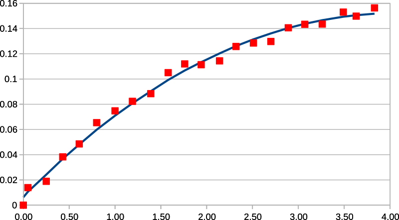
Fig. 9 Modeled Logarithmic Sensor Reading Error

Slope Correction

Applying the slope calibration coefficients to a basic count value is performed on-device, before that value is used as part of density calculations.

The process is fairly straightforward. It involves applying the polynomial calculated above to the value in a logarithmic space, then converting back to a linear space.

The inputs are as follows:

• \(B_0, B_1, B_2\): Slope calibration coefficients

• \(V_{basic}\): Sensor reading value, in basic counts

The correction itself is thus:

\begin{align*} M_{reading} &= log_{10} V_{basic} \\ M_{expected} &= B_0 + (B_1 * M_{reading}) + (B_2 * {M_{reading}}^2) \\ V_{corrected} &= 10^{M_{expected}} \end{align*}

Sensor Head Design

The sensor head is designed to support both reflection and transmission measurements from a single sensor element, using multiple light sources. It is articulated using a hinge mechanism that brings the two halves of the unit to a repeatable alignment and parallel position, when an object no thicker than a normal piece of photographic film or paper is placed in-between.

For reflection measurements, the light source consists of four light-emitting diodes (LEDs) arranged and directed so that they shine at a 45° angle to the target. This arrangement was chosen to ensure even illumination regardless of surface or alignment imperfections, and because it provides a converging cross-hair effect when positioning a material to be measured. The LEDs are driven with a constant current that is matched between all four of them to ensure even illumination.

For transmission measurements, the light source consists of a single LED positioned below a diffuser in the base of the unit. It is also driven with a constant current, and shines upwards directly towards the sensor.

The light path towards the sensor itself, within the sensor head, consists of a diffuse material followed by a UV-IR cut filter. These help even out the light from the measurement target, and reduce the impact of any residual infrared light on the sensor readings.

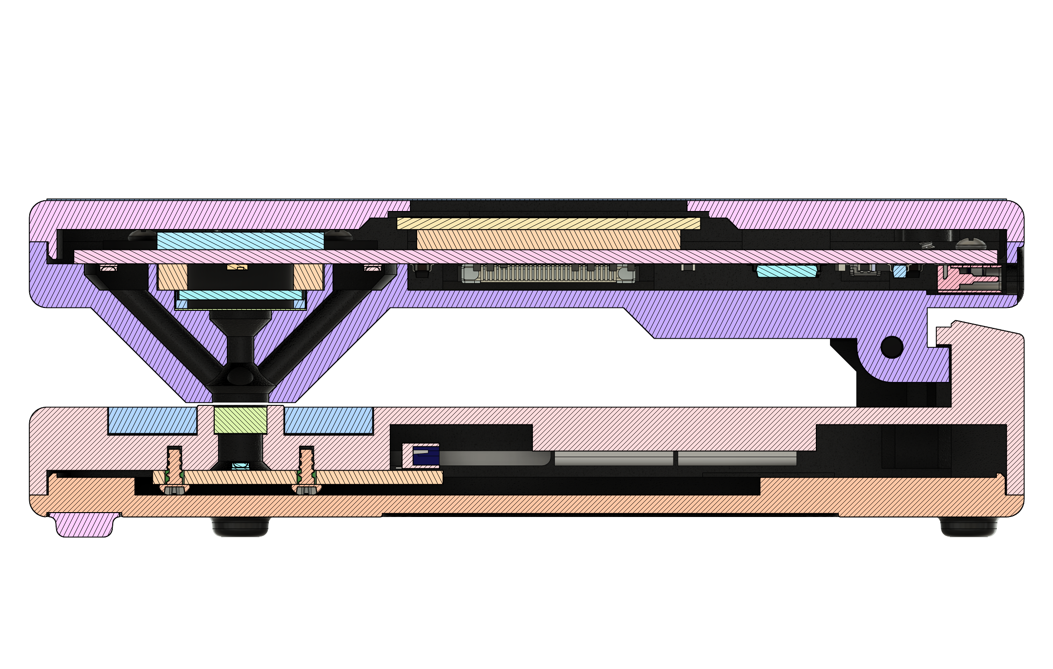
Fig. 10 Cross-section (side view)

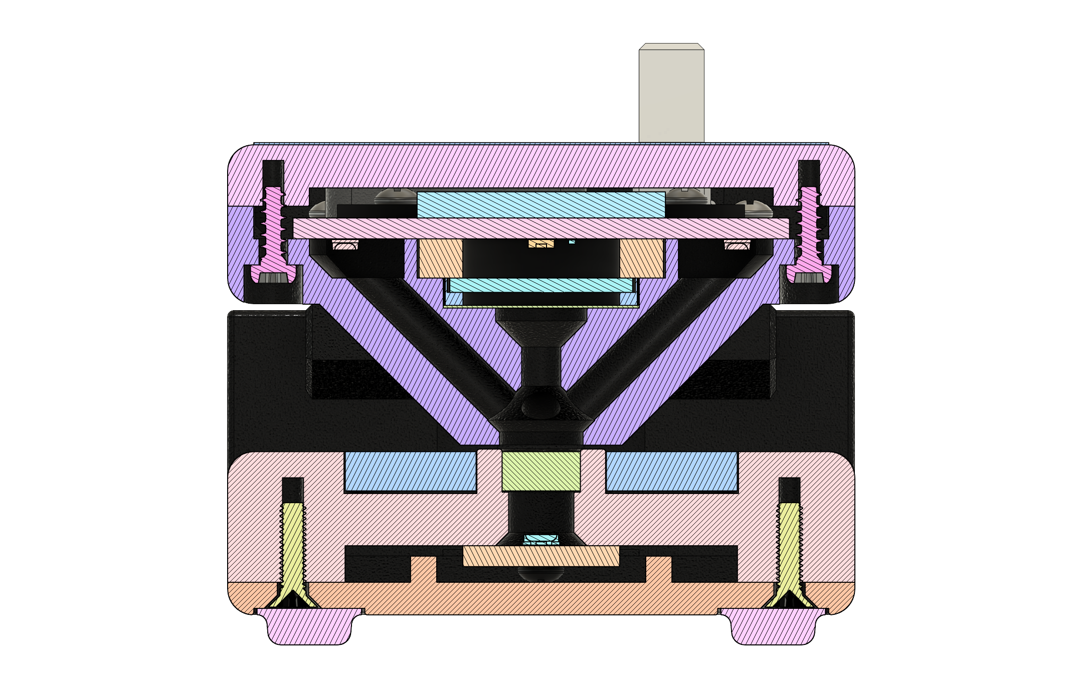
Fig. 11 Cross-section (sensor head)

Response Spectrum

The ISO specification for photographic density provides spectral conditions for each kind of density measurement. To reduce cost and increase ease of part sourcing, the sensor used in this device is an off-the-shelf component that was not designed with these conditions in mind. While it is close, it does not exactly match. That being said, when the response curve from the sensor’s datasheet is combined with the transmission curve of the UV-IR cut filter, the combined sensitivity spectrum can be seen in Fig. 12.

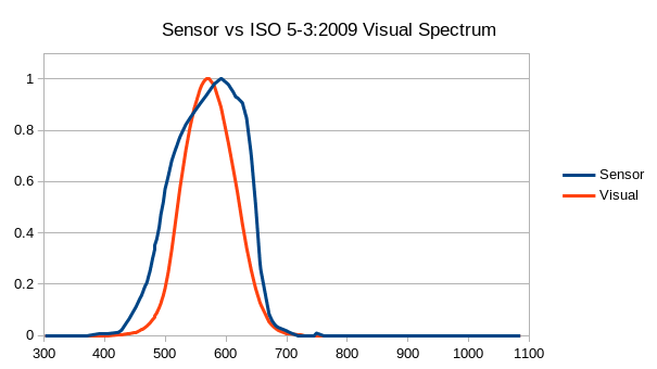
Fig. 12 Spectral response of the light sensor

It should be noted that because the sensor head’s spectral response only approximates the ISO 5-3:2009 Visual Spectrum specification, and because modern LED-based light sources do not have the same full spectrum emissions as a tungsten lamp, the most consistent results will be achieved on normal black and white photographic materials. If the measurement target has a strong shift to the blue or red side of the light spectrum, results may no longer match up.

Temperature Performance

As part of pre-production device testing, the densitometer was subjected to a wide range of thermal conditions to determine their effect on density measurements. These tests consisted of a repeatable temperature ramp from 0°C through 45°C, and were conducted with a wide range of high and low density materials secured within the device’s measurement target area. The readings were normalized around 25°C, and the measurement errors from the test can be seen in Fig. 13. The conclusion from these tests was that temperature has a very minimal effect across a reasonably large range.

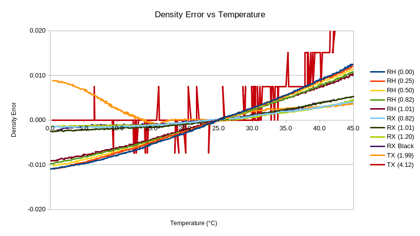
Fig. 13 Temperature sensitivity of density readings

It should be noted that the lines on this graph with the most jagged or inconsistent results were from high density transmission targets where the measurement resolution is relatively low. Due to the logarithmic nature of the scale, it would not be practical to increase the brightness of the light source by a large enough amount to compensate for this.

Footnotes

1

The ISO standards for density were preceded by the following ANSI standards: PH 2.16, PH 2.17, PH 2.18, and PH 2.19. Older product specifications are likely to cite these instead.

2

To avoid the need to calibrate the integration time, all readings are taken with the same value for this setting.

3

The “GA” and “DF” constants are only relevant for lux calculations. For the purposes of our device, they are not important as long as they do not change.

4

The method itself is described here (https://en.wikipedia.org/wiki/Least_squares), whereas the actual code used is based on this (https://www.bragitoff.com/2018/06/polynomial-fitting-c-program/) implementation.